Example: running evaluation
Here we present a tutorial on how you can use the OpenDenoising benchmark to compare the performance of denoising algorithms. You can run through this examples running the code snippets sequentially.
First, being on the project’s root, you need to import the modules provided by the OpenDenoising benchmark:
from OpenDenoising import data
from OpenDenoising import model
from OpenDenoising import evaluation
from OpenDenoising import Benchmark
To execute multiple models that access the GPU, you need to allow Tensorflow/Keras to allocate memory only when needed. This is done through,
import keras
import tensorflow as tf

# Configures Tensorflow session
config = tf.ConfigProto()
config.gpu_options.allow_growth = True
session = tf.Session(config=config)
keras.backend.set_session(session)
For now on, we suppose you are running your codes on the project root folder.
Defining Datasets
To define a dataset to evaluate your algorithms, you need to have at hand saved image files in the following folder structure:
Clean Dataset (only references)
DatasetName/
|-- Train
|   |-- ref
|-- Valid
|   |-- ref
Full Dataset (references and noisy images)
DatasetName/
|-- Train
|   |-- in
|   |-- ref
|-- Valid
|   |-- in
|   |-- ref
To run this example, you can use the data module to download test datasets,
data.download_dncnn_testsets(output_dir="./tmp/TestSets", testset="BSD68")
data.download_dncnn_testsets(output_dir="./tmp/TestSets", testset="Set12")
The previous snippet will create the entire folder structure on a temporary folder called “tmp”. Moreover to create the object for generating image samples, you can use the following commands,
# BSD Dataset
BSD68 = data.DatasetFactory.create(path="./tmp/TestSets/BSD68/",
                                   batch_size=1,
                                   n_channels=1,
                                   noise_config={data.utils.gaussian_noise: [25]},
                                   name="BSD68")
# Set12 Dataset
Set12 = data.DatasetFactory.create(path="./tmp/TestSets/Set12/",
                                   batch_size=1,
                                   n_channels=1,
                                   noise_config={data.utils.gaussian_noise: [25]},
                                   name="Set12")
datasets = [BSD68, Set12]
Defining Models
Deep Learning Models
In “./Additional Files”, you have at your disposal various pre-trained models. To load them, you only need to specify the path to the file containing their architecture/weights. For more details about how the model module works, you can look the Model module tutorial.
Bellow, we charge each model using the respective wrapper class for its framework.
# Keras rednet30
keras_rednet30 = model.KerasModel(model_name="Keras_Rednet30")
keras_rednet30.charge_model(model_path="./Additional Files/Keras Models/rednet30.hdf5")

# Keras rednet20
keras_rednet20 = model.KerasModel(model_name="Keras_Rednet20")
keras_rednet20.charge_model(model_path="./Additional Files/Keras Models/rednet20.hdf5")

# Keras rednet10
keras_rednet10 = model.KerasModel(model_name="Keras_Rednet10")
keras_rednet10.charge_model(model_path="./Additional Files/Keras Models/rednet10.hdf5")

# Onnx dncnn from Matlab
onnx_dncnn = model.OnnxModel(model_name="Onnx_DnCNN")
onnx_dncnn.charge_model(model_path="./Additional Files/Onnx Models/dncnn.onnx")
Filtering Models
The specification of filtering models is made the same way. Since these kinds of model do not need to be trained, you only need to specify the function that will perform the denoising. Bellow, we specify BM3D implemented on Python through Matlab’s engine.
Note If you have not installed Matlab support, or have not installed BM3D library from the author’s website, do not execute the next snippet.
# BM3D from Matlab
bm3d_filter = model.FilteringModel(model_name="BM3D_filter")
bm3d_filter.charge_model(model_function=model.filtering.BM3D, sigma=25.0, profile="np")
List of Models
If you have instantiated BM3D model,
models = [bm3d_filter, onnx_dncnn, keras_rednet10, keras_rednet20, keras_rednet30]
Otherwise,
models = [onnx_dncnn, keras_rednet10, keras_rednet20, keras_rednet30]
Metrics
Metrics are mathematical functions that allow the assessment of image quality. The evaluation module contains
a list of built-in metrics commonly used on image processing.
MSE
The Mean Squared Error metric is a metric used to calculate the mean deviation of pixels between two images \(y_{true}\) and \(y_{pred}\),
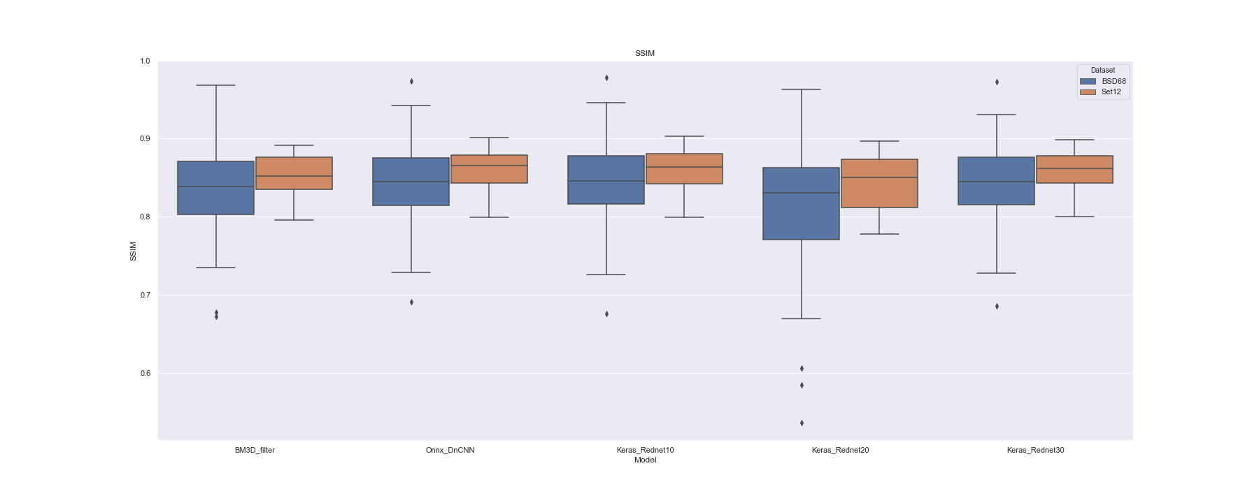
SSIM
The Structural Similarity Index is a metric that evaluates the perceived quality of a given image, with respect to a reference image. Let \(x\) and \(y\) be image patches, the SSIM between them is,
where
- \(\mu_{x}\), \(\mu_{y}\) are respectively the mean of pixels in each patch.
- \(\sigma_{x}\), \(\sigma_{y}\) are respectively the variance of pixels in each patch.
- \(\sigma_{xy}\) is the covariance between patches \(x\) and \(y\).
- \(c_{1} = 0.01\), \(c_{2} = 0.03\)
PSNR
The Peak Signal to Noise Ratio is metric used for measuring noise present on signals. Its computation is based on the MSE metric,
where \(max(y_{true})\) corresponds to the maximum pixel value on \(y_{true}\).
Creating Custom Metrics
The OpenDenoising benchmark has two types of functions: those that act on symbolic tensors, and those that act on
actual numeric arrays (from numpy). The backend used to process tensors is Tensorflow, and its functions cannot be called
directly on numpy.ndarray objects.
This introduces a double behavior on Metric functions (those that act upon tensors, and those that act upon arrays). To cope with this issue, we propose a class called “Metric”, that wraps tensorflow-based and numpy-based functions, handling when to call one or another.
For evaluation purposes, we only need to specify metrics that process numpy arrays. To define PSNR, SSIM and MSE metrics we run the following snippet,
mse_metric = evaluation.Metric(name="MSE", np_metric=evaluation.skimage_mse)
ssim_metric = evaluation.Metric(name="SSIM", np_metric=evaluation.skimage_ssim)
psnr_metric = evaluation.Metric(name="PSNR", np_metric=evaluation.skimage_psnr)

metrics = [mse_metric, psnr_metric, ssim_metric]
Visualisations
Visualisations are functions to create plots based on the evaluation results. To define a visualisation you need to
specify the function to generate the plot, and the use the class OpenDenoising.evaluation.Visualisation to
wrap it. The OpenDenoising benchmark provides box plots of default metrics as built-ins options for visualisations,
as follows,
boxplot_PSNR = evaluation.Visualisation(func=partial(evaluation.boxplot, metric="PSNR"),
                                        name="Boxplot_PSNR")

boxplot_SSIM = evaluation.Visualisation(func=partial(evaluation.boxplot, metric="SSIM"),
                                        name="Boxplot_SSIM")

boxplot_MSE = evaluation.Visualisation(func=partial(evaluation.boxplot, metric="MSE"),
                                        name="Boxplot_MSE")
visualisations = [boxplot_PSNR, boxplot_SSIM, boxplot_MSE]
Evaluation
To run an evaluation session you need to instantiate the OpenDenoising.Benchmark class, and then register
the list we have created so far (datasets, models, metrics and visualisations) through the method register, as follows,
benchmark = Benchmark(name="BSD68_Test12", output_dir='./tmp/results')

# Register metrics
benchmark.register(metrics)
# Register datasets
benchmark.register(datasets)
# Register models
benchmark.register(models)
# Register visualisations
benchmark.register(visualisations)

benchmark.evaluate()
This snippet has as output:


All evaluation results are saved on ‘./tmp/results/BSD68_Test12’ folder, which was specified by output_dir and name. There you may find two .csv files (partial_results.csv and general_results.csv). partial_results.csv holds the denoising results for each image present on each dataset, for each model, and general_results holds statistics for model and dataset (mean and variance).